


Clustering is one of the most common tools for exploring structure in data. It helps reveal groups, patterns, and relationships that are not obvious from raw tables or summary statistics. Among clustering methods, k-means is often the default choice, but it is not always the most appropriate one. K-medoids clustering is a practical and more robust alternative, especially when working with outlier-prone, heterogeneous, or non-Euclidean data.
This article introduces the core ideas behind k-medoids clustering, explains how it differs from k-means and other approaches, and outlines when it is worth considering in applied data science work.
The core idea behind K-medoids
At a high level, k-medoids clustering partitions data into k groups, just like k-means. The key difference lies in how each cluster is represented. Instead of using the mean of the points in a cluster, k-medoids chooses an actual data point as the cluster representative. This representative is called the medoid.
The medoid is whichever point in a cluster has the lowest total distance to the rest. Because it must be a real observation, the medoid always corresponds to a valid and interpretable data record.
Figure 1 puts these two representatives side by side. It marks two points for one group of observations, the mean that k-means would use and the medoid that k-medoids would use. Add an extreme observation and drag it away from the group to see what happens.
Figure 1 · robustness
How the mean and the medoid respond to an extreme observation
The mean is a computed point that can drift toward an extreme value. The medoid is an actual observation chosen to minimize total distance, so it tends to stay with the bulk of the data. Add an extreme observation and move it outward to compare the two.
Interactive figure. A group of ten observations is shown on a scatter plot with average session length in minutes on the horizontal axis and sessions per week on the vertical axis. A mean marker and a medoid marker are drawn. A control adds one extreme observation and a slider moves it further from the group. As the extreme observation moves out, the mean marker follows it while the medoid marker stays on a central observation. With the extreme observation at the far position, the mean moves to about 32, 22 while the medoid remains on observation P2 at 26, 18.
Interactive controls need JavaScript. The scene above shows the fixed result. The mean marker sits away from the group toward the extreme observation, while the medoid marker stays on a central observation.
The two objectives measure different quantities and are not directly comparable. Squared distances grow faster than distances, which is why the k‑means objective reacts more sharply to the extreme observation. The medoid resists movement, yet its objective still rises, so robustness softens the effect of an extreme value while leaving it in place.
Figure 1. The mean and the medoid for one group of observations. As the extreme observation moves outward, the mean drifts toward it while the medoid stays on a central data point.
The medoid holds its position because moving to the extreme observation would increase its total distance to the rest of the group. That resistance is the root of the robustness that sets k-medoids apart from k-means, which the next section examines in more detail.
K-medoids versus K-means
K-means minimizes the sum of squared Euclidean distances between points and their assigned cluster centroids, which is computationally efficient and easy to implement, though it leaves the method sensitive to outliers. A single extreme value can pull a centroid far away from the bulk of the data and distort cluster assignments.
K-medoids, by contrast, minimizes the sum of distances from each point to its nearest medoid. Because distances are not squared and the representative cannot leave the data, an extreme value pulls that representative far less. The outlier still joins a cluster and still counts toward the objective. What it cannot do is drag the representative far.
Another practical difference concerns distance metrics. K-means is fundamentally tied to Euclidean distance and the notion of an average. K-medoids can be used with any distance or dissimilarity measure, including Manhattan distance, cosine distance, or even precomputed distance matrices. That freedom suits data types where averages are not meaningful, such as categorical variables, mixed feature spaces, or complex similarity measures.
Figure 2 makes the effect of the distance choice concrete. It clusters a small set of customers described by annual spend and an engagement score, and it lets you switch the feature scaling and the distance metric to watch the clusters and their medoids respond.
Figure 2 · dissimilarity and scaling
The distance you choose decides which observations count as similar
K‑medoids can run on any dissimilarity. This example clusters thirteen customers described by annual spend and an engagement score. Switch the feature scaling and the distance metric to see how the two clusters and their medoids change.
Interactive figure. Thirteen observations are plotted in standardized coordinates, with standardized spend on the horizontal axis and standardized engagement on the vertical axis. Controls switch the feature scaling between raw units and standardized, and switch the distance metric between Euclidean and Manhattan. With raw units the two clusters split by spend from left to right, because spend has a much larger numeric range. After standardizing, the clusters split by engagement into a high band and a low band. One observation, P13, sits between the two bands, and its cluster depends on the metric: Euclidean places it in the low engagement cluster, Manhattan places it in the high engagement cluster.
Interactive controls need JavaScript. The scene above shows standardized Euclidean clustering, where the observations separate into a high engagement band and a low engagement band.
After standardizing, spend and engagement contribute on the same scale. The clusters separate into a high engagement band and a low engagement band.
| Medoid | Distance |
|---|---|
| Medoid P4 · Cluster 1 (blue) | 1.0 |
| Medoid P9 · Cluster 2 (amber) | 0.9 |
Observation P13 sits between the two bands. Under Euclidean distance it joins Cluster 2. Beyond the two metrics offered here, k‑medoids also accepts cosine distance or a precomputed dissimilarity matrix, so the metric is worth choosing deliberately to match the data.
Figure 2. K-medoids applied to thirteen customers under two feature-scaling choices and two distance metrics. In raw units, spend spans thousands while engagement spans single digits, so distance is dominated by spend and the clusters split by spend. After standardizing, the two features contribute equally and the clusters split by engagement. Observation P13 lies between the engagement bands, and the metric decides which cluster it joins.
The dissimilarity you supply defines what counts as similar, so feature scaling and metric selection are modeling decisions in their own right. For this data, scaling changes the whole partition, while the choice between Euclidean and Manhattan distance moves only the ambiguous observation between clusters.
Comparison with other clustering methods
Compared to hierarchical clustering, k-medoids offers the same flexibility in distance definitions, and its advantage lies there rather than in scaling. Classical PAM compares every medoid with every non-medoid on each swap pass, which is comparable to agglomerative methods or heavier. It is variants such as Clustering Large Applications (CLARA) and Clustering Large Applications based on RANdomized Search (CLARANS) that scale to larger datasets. Hierarchical methods provide rich structure but can become computationally expensive and harder to tune in practice.
Density-based methods like DBSCAN focus on discovering arbitrarily shaped clusters and identifying noise points. These methods shine when cluster density is the primary signal. They also demand careful parameter choices, and they falter when densities vary widely. K-medoids, by contrast, hands back a clear partition into a fixed number of clusters. Exploratory analysis and downstream modeling both tend to want exactly that.
Model-based approaches such as Gaussian mixture models rely on distributional assumptions that may not hold in real data. K-medoids makes no distributional assumption and works purely from distances between observations. That does not make it assumption-free. Like k-means it looks for a fixed number of compact groups around single representatives, so elongated or nested shapes stay out of reach.
Practical advantages of K-medoids
One of the strongest advantages of k-medoids is robustness. The objective sums unsquared distances, and the representative has to be an actual observation. Together those two facts blunt the effect of noise and extreme values, without removing it. The outlier still joins a cluster and still counts toward the objective. That robustness is what recommends the method in domains like finance, healthcare, and behavioral data, where outliers are common and often meaningful.
Interpretability is another benefit. A medoid can be inspected directly, summarized, or used as a representative example of a cluster. Stakeholders tend to follow that more easily than an abstract centroid sitting where no real data point does.
Freedom over the distance metric widens the range of applications. Define a sensible dissimilarity measure and k-medoids will run on it.
Cost, scale and choosing k
Cost is the trade. Finding optimal medoids means evaluating a great many pairwise distances, which grows with the size of the dataset. Modern implementations and heuristics narrow the gap, and k-medoids runs slower than k-means.
Scalability is the next question. Very large datasets are handled with approximate methods or sampling. For a first look, k-means or a mini-batch variant is the lighter option.
Finally, like k-means, k-medoids requires specifying the number of clusters in advance, which puts weight on model selection, often supported by validation metrics such as silhouette scores or stability analyses.
Figure 3 shows where the computational cost comes from. It walks through Partitioning Around Medoids, usually shortened to PAM, the classic algorithm for k-medoids. The walkthrough covers two phases. Build picks an initial set of medoids. Swap then tests exchanging a medoid for another observation, keeping only the exchanges that lower the total distance.
Figure 3 · the PAM algorithm
How partitioning around medoids searches for the medoids
PAM first builds an initial set of medoids, then repeatedly tests swapping a medoid for a non‑medoid and keeps only swaps that lower the total distance. Play the walkthrough, or step through it, to follow the build and swap phases.
Interactive figure. Twelve observations are plotted on a scatter plot and grouped into two clusters. The build phase picks the observation with the lowest total distance to all points as the first medoid. It then adds whichever observation lowers the total distance most as the second. In the swap phase it evaluates twenty candidate swaps, each replacing one medoid with one non‑medoid, and applies the swap that most lowers the total distance. After one accepted swap the medoids settle on observations P5 and P8, the total distance is 123.4, and no further swap lowers it, so the algorithm stops at a local optimum. Controls play, pause, step forward, step back, and reset the walkthrough.
Interactive controls need JavaScript. The scene above shows the final result, where PAM has settled on the two medoids that give the lowest total distance it can reach by local swaps.
This is classical PAM. The swap phase is a local search, so the result can depend on the starting medoids and is not guaranteed to be the global optimum. Each pass evaluates every medoid against every non‑medoid, which is the source of PAM’s cost. FastPAM and FasterPAM reach the same objective more quickly. CLARA and CLARANS go further and scale to larger datasets, by limiting how much of the problem they search at once.
Figure 3. One run of PAM on twelve observations with k set to two. The build phase picks the first medoid as the observation with the lowest total distance to all points, then adds a second medoid. The swap phase evaluates every medoid against every non-medoid and applies the exchange that most lowers the total distance. The run stops when no exchange improves the objective.
Each swap pass compares every medoid with every non-medoid, which is why PAM becomes costly as the dataset grows. The search is local, so the outcome depends on the starting medoids and is not guaranteed to reach the lowest possible total distance.
Example: K-medoids clustering for customer data
K-MedoidsSegments
How K-Medoids turns nearly 9,000 credit card customers into behavioral segments anchored by real cardholders. The data are imputed, standardized, validated and profiled.
K-Medoids Segments. How K-Medoids turns nearly 9,000 credit card customers into behavioral segments anchored by real cardholders. The data are imputed, standardized, validated and profiled. Key topics covered: Credit card customer data, Impute missing values, Clusters in principal component analysis (PCA) space, Standardize features, Fit K-Medoids, Profile each segment, Interactive 3D view, Choose the number of clusters.
In this example, we will build a customer segmentation model using credit card transaction and behavior data.
Our main business goal is to:
- Group credit card customers into behavioral segments (clusters)
- Help marketing and product teams design targeted strategies for each segment
We will:
- Use K-Medoids clustering to segment customers
- Choose the number of clusters using the silhouette score, with two further indices reported alongside it
- Use PCA (Principal Component Analysis) to visualize clusters in 2D and 3D
- Create a descriptive Table 1 stratified by cluster using the
tableonepackage
The dataset (CC GENERAL.csv) contains ~9,000 customers and 18 columns, of which 17 are behavioral variables once the CUST_ID identifier is dropped.
Imports and configuration
In this section we:
- Import all necessary Python libraries
- Configure plotting styles for nicer visuals
- Optionally suppress non-critical warnings to keep the notebook output clean
import numpy as np
import pandas as pd

import matplotlib.pyplot as plt
import seaborn as sns
import plotly.graph_objects as go

from sklearn.experimental import enable_iterative_imputer
from sklearn.preprocessing import StandardScaler
from sklearn.decomposition import PCA

from sklearn.metrics import (
    silhouette_score,
    calinski_harabasz_score,
    davies_bouldin_score,
)

from joblib import Parallel, delayed
import multiprocessing

from pyclustering.cluster.kmedoids import kmedoids
from pyclustering.utils.metric import distance_metric, type_metric
from tableone import TableOne

# ============================================================
# Global configuration
# ============================================================
RANDOM_STATE = 42

sns.set(style="whitegrid", context="notebook")
plt.rcParams["figure.figsize"] = (10, 6)
plt.rcParams["axes.titlesize"] = 14
plt.rcParams["axes.labelsize"] = 12
K-medoids wrapper class
Define a minimal, sklearn-like interface for K-Medoids using pyclustering.
# ============================================================
# K-Medoids using pyclustering
# ============================================================

class KMedoids:
    """
    Minimal sklearn-like K-Medoids wrapper using pyclustering.
    """

    def __init__(
        self,
        n_clusters,
        metric="euclidean",
        init="random",
        random_state=None,
    ):
        self.n_clusters = int(n_clusters)
        self.metric = metric
        self.init = init
        self.random_state = random_state

        self.labels_ = None
        self.medoid_indices_ = None

    def _get_metric(self):
        if self.metric == "manhattan":
            return distance_metric(type_metric.MANHATTAN)
        return distance_metric(type_metric.EUCLIDEAN)

    def _init_medoids(self, n_samples):
        rng = np.random.RandomState(self.random_state)
        return rng.choice(
            n_samples,
            size=self.n_clusters,
            replace=False,
        ).tolist()

    def fit(self, X):
        X = np.asarray(X)
        n_samples = X.shape[0]

        initial_medoids = self._init_medoids(n_samples)
        metric = self._get_metric()

        model = kmedoids(
            data=X.tolist(),
            initial_index_medoids=initial_medoids,
            metric=metric,
        )
        model.process()

        clusters = model.get_clusters()
        medoids = model.get_medoids()

        labels = np.empty(n_samples, dtype=int)
        for cluster_id, indices in enumerate(clusters):
            labels[indices] = cluster_id

        self.labels_ = labels
        self.medoid_indices_ = np.asarray(medoids, dtype=int)

        return self

    def fit_predict(self, X):
        self.fit(X)
        return self.labels_
Load and inspect the data
We now load the CC GENERAL.csv file and take a first look at basic descriptive statistics of the dataset.
# Load the dataset
data_path = "CC GENERAL.csv"
df = pd.read_csv(data_path)

# Descriptive statistics for numerical columns
print("\nDescriptive statistics for numerical variables:")
desc_stats = df.describe().T.round(2)
display(desc_stats)

# Save descriptive statistics as CSV
desc_stats.to_csv("descriptive_statistics.csv")Descriptive statistics for numerical variables:Descriptive statistics for the 17 variables
| count | mean | std | min | 25% | 50% | 75% | max | |
|---|---|---|---|---|---|---|---|---|
| BALANCE | 8950.0 | 1564.47 | 2081.53 | 0.00 | 128.28 | 873.39 | 2054.14 | 19043.14 |
| BALANCE_FREQUENCY | 8950.0 | 0.88 | 0.24 | 0.00 | 0.89 | 1.00 | 1.00 | 1.00 |
| PURCHASES | 8950.0 | 1003.20 | 2136.63 | 0.00 | 39.64 | 361.28 | 1110.13 | 49039.57 |
| ONEOFF_PURCHASES | 8950.0 | 592.44 | 1659.89 | 0.00 | 0.00 | 38.00 | 577.40 | 40761.25 |
| INSTALLMENTS_PURCHASES | 8950.0 | 411.07 | 904.34 | 0.00 | 0.00 | 89.00 | 468.64 | 22500.00 |
| CASH_ADVANCE | 8950.0 | 978.87 | 2097.16 | 0.00 | 0.00 | 0.00 | 1113.82 | 47137.21 |
| PURCHASES_FREQUENCY | 8950.0 | 0.49 | 0.40 | 0.00 | 0.08 | 0.50 | 0.92 | 1.00 |
| ONEOFF_PURCHASES_FREQUENCY | 8950.0 | 0.20 | 0.30 | 0.00 | 0.00 | 0.08 | 0.30 | 1.00 |
| PURCHASES_INSTALLMENTS_FREQUENCY | 8950.0 | 0.36 | 0.40 | 0.00 | 0.00 | 0.17 | 0.75 | 1.00 |
| CASH_ADVANCE_FREQUENCY | 8950.0 | 0.14 | 0.20 | 0.00 | 0.00 | 0.00 | 0.22 | 1.50 |
| CASH_ADVANCE_TRX | 8950.0 | 3.25 | 6.82 | 0.00 | 0.00 | 0.00 | 4.00 | 123.00 |
| PURCHASES_TRX | 8950.0 | 14.71 | 24.86 | 0.00 | 1.00 | 7.00 | 17.00 | 358.00 |
| CREDIT_LIMIT | 8949.0 | 4494.45 | 3638.82 | 50.00 | 1600.00 | 3000.00 | 6500.00 | 30000.00 |
| PAYMENTS | 8950.0 | 1733.14 | 2895.06 | 0.00 | 383.28 | 856.90 | 1901.13 | 50721.48 |
| MINIMUM_PAYMENTS | 8637.0 | 864.21 | 2372.45 | 0.02 | 169.12 | 312.34 | 825.49 | 76406.21 |
| PRC_FULL_PAYMENT | 8950.0 | 0.15 | 0.29 | 0.00 | 0.00 | 0.00 | 0.14 | 1.00 |
| TENURE | 8950.0 | 11.52 | 1.34 | 6.00 | 12.00 | 12.00 | 12.00 | 12.00 |
Data preprocessing
Before clustering, we need to:
- Remove the identifier column (
CUST_ID) from the feature set - Inspect and handle missing values
- Construct a clean numerical feature matrix
Xsuitable for downstream scaling and clustering
We first examine the extent of missingness in each column to understand which variables require imputation. The identifier column (CUST_ID) is excluded from the feature matrix, as it does not carry meaningful information for clustering.
Handling missing values
Rather than using univariate imputation, we apply a model-based multivariate imputation strategy using IterativeImputer with a BayesianRidge estimator. This approach:
- Models each feature with missing values as a function of the other features
- Iteratively refines imputations over multiple rounds until convergence
- Approximates multivariate relationships between variables, which is especially important for clustering
import pandas as pd
from sklearn.impute import IterativeImputer
from sklearn.linear_model import BayesianRidge

# Keep a copy of the original dataframe with CUST_ID for later interpretation
df_original = df.copy()

# Check missing values per column
print("Missing values per column:")
missing_counts = df.isna().sum().sort_values(ascending=False)
display(missing_counts)

# Drop CUST_ID from the features (identifier, not used for clustering)
if "CUST_ID" in df.columns:
    df_features = df.drop(columns=["CUST_ID"])
else:
    df_features = df.copy()

# Feature matrix (numerical variables)
X = df_features.copy()

# Model-based multivariate imputer
imputer = IterativeImputer(
    estimator=BayesianRidge(),
    max_iter=20,
    tol=1e-3,
    imputation_order="ascending",
    random_state=42
)

# Fit and transform
X_imputed = imputer.fit_transform(X)

# Convert back to DataFrame
X_imputed = pd.DataFrame(
    X_imputed,
    columns=X.columns,
    index=X.index
)
Missing values per column:MINIMUM_PAYMENTS 313
CREDIT_LIMIT 1
BALANCE 0
CUST_ID 0
BALANCE_FREQUENCY 0
PURCHASES 0
CASH_ADVANCE 0
PURCHASES_FREQUENCY 0
ONEOFF_PURCHASES 0
INSTALLMENTS_PURCHASES 0
PURCHASES_INSTALLMENTS_FREQUENCY 0
ONEOFF_PURCHASES_FREQUENCY 0
CASH_ADVANCE_TRX 0
CASH_ADVANCE_FREQUENCY 0
PURCHASES_TRX 0
PAYMENTS 0
PRC_FULL_PAYMENT 0
TENURE 0
dtype: int64Note on distribution and skewness
Many financial variables (e.g., BALANCE, PURCHASES, CASH_ADVANCE) are typically
right-skewed with long tails. For simplicity and interpretability, we will:
- Leave the data in its original scale, but
- Apply standardization before k-medoids (which works on distances)
In a more advanced analysis, we might consider log-transforming highly skewed variables before scaling, but we will not do that here to keep the workflow straightforward.
Feature scaling
K-Means is a distance-based algorithm that uses squared Euclidean distances, and k-medoids is distance-based too, whatever measure it is given. Variables on larger scales (e.g., dollars) can dominate others (e.g., frequencies mostly in [0, 1], though CASH_ADVANCE_FREQUENCY reaches 1.50).
Therefore, we:
- Use
StandardScalerto standardize each feature:- Mean = 0
- Standard deviation = 1
This lets all variables contribute more equally to the clustering.
K-Medoids is also distance-based, so scaling remains important. Because medoids must be actual observations, K-Medoids is often more robust to outliers than K-Means, but it still relies on meaningful distances between features.
scaler = StandardScaler()
X_scaled = scaler.fit_transform(X_imputed)

print("Shape of scaled feature matrix:", X_scaled.shape)Shape of scaled feature matrix: (8950, 17)Selecting the number of clusters (choosing k for K-medoids)
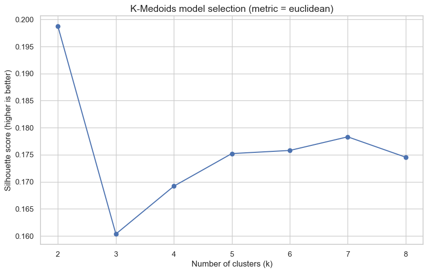
Unlike K-Means, K-Medoids does not optimize a “within-cluster dispersion” objective in the same way, so the k-means elbow plot of within-cluster sum of squares does not carry over directly. An elbow on the k-medoids objective is possible, but it is not the route taken here to select k.
Instead, we evaluate a range of k values using cluster validity indices:
- Silhouette score (primary): higher is better (balance of cohesion and separation)
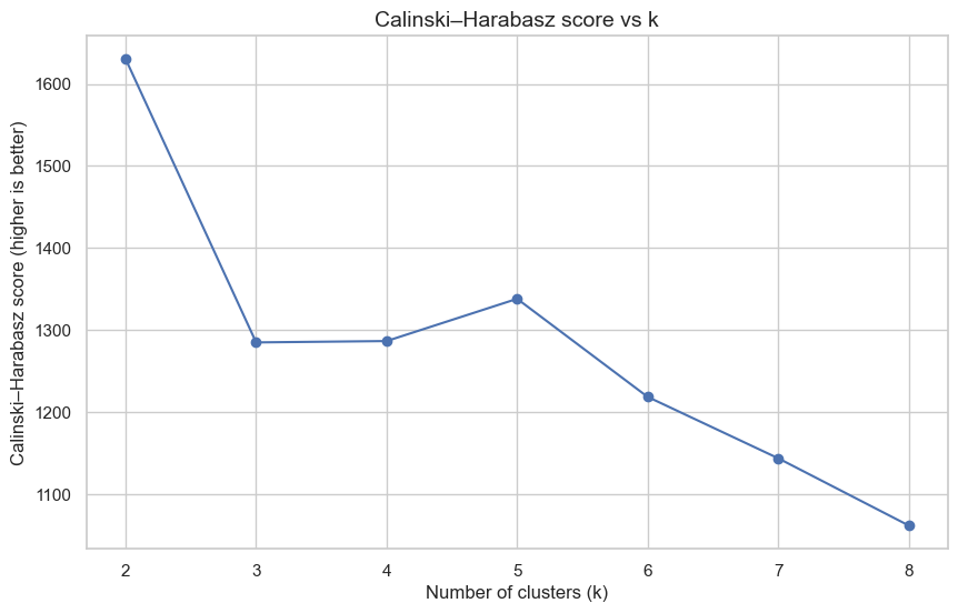
- Calinski–Harabasz score (secondary): higher is better
- Davies–Bouldin score (secondary): lower is better
We will fit K-Medoids across a reasonable range of k values and select a final k based on the evidence from these metrics.
# Range of k values to try (keep runtime reasonable)
k_values = list(range(2, 9))

# Distance metric for K-Medoids
DIST_METRIC = "euclidean"

# Use all CPU cores
N_JOBS = multiprocessing.cpu_count()


def evaluate_k(k, X, metric, random_state):
    """
    Fit K-Medoids for a given k and compute validation metrics.
    Returns (k, silhouette, calinski_harabasz, davies_bouldin).
    """
    kmed = KMedoids(
        n_clusters=k,
        metric=metric,
        init="k-medoids++",  # kept for API compatibility
        random_state=random_state,
    )
    labels = kmed.fit_predict(X)

    sil = silhouette_score(X, labels, metric=metric)
    ch = calinski_harabasz_score(X, labels)
    db = davies_bouldin_score(X, labels)

    return k, sil, ch, db


# Run evaluations in parallel (each k is independent)
results = Parallel(n_jobs=N_JOBS, backend="loky")(
    delayed(evaluate_k)(k, X_scaled, DIST_METRIC, RANDOM_STATE)
    for k in k_values
)

# Unpack results (sort by k to keep plots ordered)
results = sorted(results, key=lambda t: t[0])
k_vals, sil_scores, ch_scores, db_scores = map(list, zip(*results))


# ============================================================
# Plot validation metrics vs k
# ============================================================

plt.figure()
plt.plot(k_vals, sil_scores, marker="o")
plt.xticks(k_vals)
plt.xlabel("Number of clusters (k)")
plt.ylabel("Silhouette score (higher is better)")
plt.title(f"K-Medoids model selection (metric = {DIST_METRIC})")
plt.grid(True)
plt.savefig("kmedoids_silhouette.png", dpi=300, bbox_inches="tight")
plt.show()

plt.figure()
plt.plot(k_vals, ch_scores, marker="o")
plt.xticks(k_vals)
plt.xlabel("Number of clusters (k)")
plt.ylabel("Calinski–Harabasz score (higher is better)")
plt.title("Calinski–Harabasz score vs k")
plt.grid(True)
plt.savefig("kmedoids_calinski_harabasz.png", dpi=300, bbox_inches="tight")
plt.show()

plt.figure()
plt.plot(k_vals, db_scores, marker="o")
plt.xticks(k_vals)
plt.xlabel("Number of clusters (k)")
plt.ylabel("Davies–Bouldin score (lower is better)")
plt.title("Davies–Bouldin score vs k")
plt.grid(True)
plt.savefig("kmedoids_davies_bouldin.png", dpi=300, bbox_inches="tight")
plt.show()Silhouette score against the number of clusters
Calinski-Harabasz score against the number of clusters
Davies-Bouldin score against the number of clusters
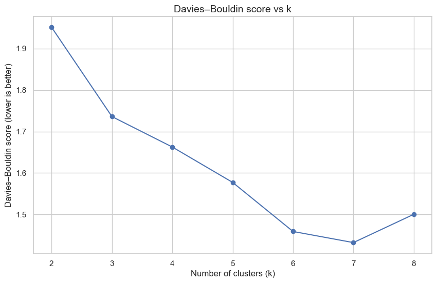
Based on the validation curves above, we select a value of k that gives the best silhouette score while keeping the solution reasonably simple. The separation itself is weak. Every silhouette score in the sweep sits between 0.16 and 0.20 on a scale that runs from -1 to 1. Calinski-Harabasz peaks at the same value, and it comes from the same fits on the same features. Davies-Bouldin, which is minimized, bottoms out at k = 7 and places the selected k at the other end. The silhouette drives the selection, and the value it picks is the smallest in the searched range, so the optimum sits on the boundary of the sweep.
In practice, Silhouette score is a solid default choice for distance-based clustering on standardized continuous features. Note that the wrapper’s initialization draws its medoids at random and does not apply k-medoids++, despite the init argument passed at both call sites, so the sweep above and the final fit below both start from random medoids at random_state=42. The code below selects the k with the best silhouette score.
# Choose k based on the best silhouette score (primary), with a bias toward simpler solutions
sil_series = pd.Series(sil_scores, index=list(k_values))
best_sil = sil_series.max()

# All k values within a tiny tolerance of the best silhouette
tol = 1e-6
candidate_ks = sil_series[sil_series >= best_sil - tol].index.tolist()
optimal_k = int(min(candidate_ks))

print(f"Selected k = {optimal_k} using silhouette score (metric = {DIST_METRIC}).")
Selected k = 2 using silhouette score (metric = euclidean).Fit final K-medoids model
With optimal_k chosen, we now:
- Fit a final
KMedoidsmodel on the scaled features - Obtain cluster labels for each customer
- Attach the cluster labels back to the original dataframe (
df_clustered) - Inspect how many customers fall into each cluster
# Fit final K-Medoids model
kmedoids_final = KMedoids(
    n_clusters=optimal_k,
    metric=DIST_METRIC,
    init="k-medoids++",
    random_state=RANDOM_STATE
)
cluster_labels = kmedoids_final.fit_predict(X_scaled)

# Medoids are representative REAL observations (indices into the input array order)
medoid_indices = kmedoids_final.medoid_indices_

# Attach cluster labels to the original dataframe
df_clustered = df_original.copy()
df_clustered["cluster"] = cluster_labels

# Show cluster sizes
print("Cluster label counts:")
display(df_clustered["cluster"].value_counts().sort_index())

print("Medoid indices (row positions in the clustered matrix):")
display(pd.Series(medoid_indices, name="medoid_row_position"))
Cluster label counts:

cluster
0    4955
1    3995
Name: count, dtype: int64

Medoid indices (row positions in the clustered matrix):
0    7063
1    7721
Name: medoid_row_position, dtype: int64
Each customer is now assigned to one of the k clusters using K-Medoids (0 to k-1).
These clusters represent behavioral customer segments, which we will further
explore using visualization and descriptive statistics.
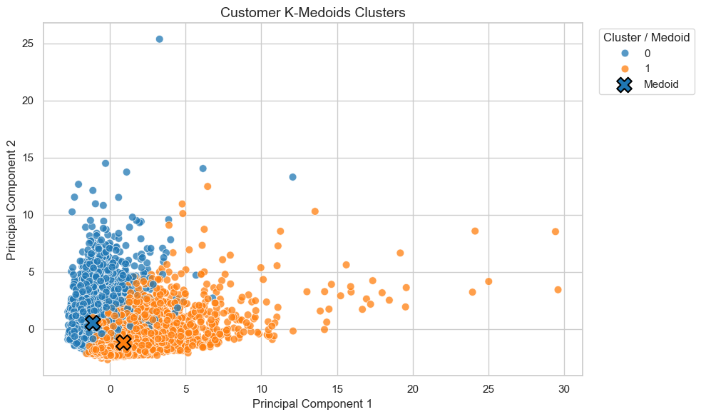
Visualizing clusters with PCA
The dataset has many dimensions (17 behavioral features), which makes it hard to visualize clusters directly. To address this, we use:
- Principal Component Analysis (PCA) to reduce the standardized features to 3 principal components
- Then plot customers in the 2D and 3D PCA space, colored by their cluster
PCA helps capture as much variance as possible in a low-dimensional projection, giving us an approximate but informative visual representation of the clusters.
# Perform PCA to reduce to 3 principal components (for visualization only)
pca = PCA(n_components=3, random_state=RANDOM_STATE)
X_pca = pca.fit_transform(X_scaled)

# Create a DataFrame for PCA results
df_pca = pd.DataFrame(
    X_pca,
    columns=["PC1", "PC2", "PC3"],
    index=df_clustered.index
)
df_pca["cluster"] = df_clustered["cluster"].astype(int)

# Mark medoids (medoids are actual observations)
df_pca["is_medoid"] = False
medoid_df_indices = df_clustered.index[medoid_indices]  # map row positions -> df index
df_pca.loc[medoid_df_indices, "is_medoid"] = True

# ----------------------------
# 2D (Seaborn/Matplotlib): medoids colored by their cluster
# ----------------------------
palette = sns.color_palette("tab10", n_colors=int(df_pca["cluster"].nunique()))
cluster_to_color = {cl: palette[i] for i, cl in enumerate(sorted(df_pca["cluster"].unique()))}

plt.figure()
sns.scatterplot(
    data=df_pca,
    x="PC1",
    y="PC2",
    hue="cluster",
    palette=cluster_to_color,
    alpha=0.75,
    s=60
)

# Overlay medoids with marker "X" but color-matched to cluster
d_m = df_pca[df_pca["is_medoid"]]
plt.scatter(
    d_m["PC1"],
    d_m["PC2"],
    s=220,
    marker="X",
    c=[cluster_to_color[c] for c in d_m["cluster"].tolist()],
    edgecolor="black",
    linewidth=1.5,
    label="Medoid"
)

plt.title("Customer K-Medoids Clusters")
plt.xlabel("Principal Component 1")
plt.ylabel("Principal Component 2")
plt.legend(title="Cluster / Medoid", bbox_to_anchor=(1.02, 1), loc="upper left")
plt.tight_layout()
plt.savefig("pca_2d_clusters_kmedoids.png", dpi=300, bbox_inches="tight")
plt.show()

# ----------------------------
# 3D (Plotly): medoids colored by their cluster
# ----------------------------
fig = go.Figure()

# Use the same tab10 mapping for Plotly (as rgb strings)
def rgb_str(rgb_tuple):
    r, g, b = rgb_tuple
    return f"rgb({int(r*255)},{int(g*255)},{int(b*255)})"

cluster_to_color_plotly = {cl: rgb_str(col) for cl, col in cluster_to_color.items()}

# Add each cluster as a separate trace (for an explicit legend)
for cl in sorted(df_pca["cluster"].unique()):
    d = df_pca[df_pca["cluster"] == cl]
    fig.add_trace(
        go.Scatter3d(
            x=d["PC1"],
            y=d["PC2"],
            z=d["PC3"],
            mode="markers",
            name=f"Cluster {cl}",
            marker=dict(
                size=4,
                opacity=0.75,
                color=cluster_to_color_plotly[cl],
            ),
        )
    )

# Add medoids as separate traces per cluster so their color matches
for cl in sorted(df_pca.loc[df_pca["is_medoid"], "cluster"].unique()):
    dmc = df_pca[(df_pca["is_medoid"]) & (df_pca["cluster"] == cl)]
    fig.add_trace(
        go.Scatter3d(
            x=dmc["PC1"],
            y=dmc["PC2"],
            z=dmc["PC3"],
            mode="markers",
            name=f"Medoid (Cluster {cl})",
            marker=dict(
                size=10,
                symbol="diamond",
                opacity=1.0,
                color=cluster_to_color_plotly[cl],
                line=dict(width=2, color="black"),
            ),
        )
    )

fig.update_layout(
    title="K-Medoids Clusters",
    scene=dict(
        xaxis_title="PC1",
        yaxis_title="PC2",
        zaxis_title="PC3",
    ),
    legend_title_text="Cluster",
)
fig.write_html("pca_3d_clusters_kmedoids_nt.html")
fig.show()

# Explained variance information
explained_var = pca.explained_variance_ratio_
print(
    f"Explained variance by PC1, PC2, PC3: {explained_var[0]:.2%}, {explained_var[1]:.2%}, {explained_var[2]:.2%}"
)
Customer clusters in the first two principal components
Interactive view of the clusters in three components
Explained variance by PC1, PC2, PC3: 27.30%, 20.32%, 8.83%Descriptive Statistics by Cluster (Table 1 using tableone)
To understand what makes each cluster unique, we will:
- Use the
tableonepackage to create a Table 1 of descriptive statistics - Stratify the table by
cluster - Include the main behavioral numeric variables (e.g., balances, purchases, cash advances)
The table helps us attach business meaning to each segment, such as:
- High spenders
- Frequent revolvers (carry a balance)
- Cash-advance heavy users
- Low-activity or dormant customers
Note: If
tableoneis not installed in your environment, you can install it via:
pip install tableone
# Prepare variables for Table 1
# We will include all numeric behavioral variables and stratify by 'cluster'.
# Exclude 'cluster' itself and the identifier 'CUST_ID' from the summarized columns.

# Identify numeric columns
numeric_columns = df_clustered.select_dtypes(include=[np.number]).columns.tolist()

# Remove 'cluster' from the list of summarized variables
if "cluster" in numeric_columns:
    numeric_columns.remove("cluster")

columns = numeric_columns
categorical = []  # No categorical variables in this example

# Create the TableOne object, stratified by cluster
table1 = TableOne(
    df_clustered,
    columns=columns,
    categorical=categorical,
    groupby="cluster",
    label_suffix=True
)

print("Table 1: Descriptive statistics of customer behavior by cluster")
display(table1)

# Save Table 1 to CSV
table1.to_csv("table1_customer_behavior_by_cluster.csv")Table 1: Descriptive statistics of customer behavior by clusterCustomer behavior summarized by cluster
| Grouped by cluster | |||||
|---|---|---|---|---|---|
| Missing | Overall | 0 | 1 | ||
| n | 8950 | 4955 | 3995 | ||
| BALANCE, mean (SD) | 0 | 1564.5 (2081.5) | 1937.4 (2222.7) | 1101.9 (1787.1) | |
| BALANCE_FREQUENCY, mean (SD) | 0 | 0.9 (0.2) | 0.9 (0.3) | 0.9 (0.2) | |
| PURCHASES, mean (SD) | 0 | 1003.2 (2136.6) | 333.1 (781.6) | 1834.3 (2867.6) | |
| ONEOFF_PURCHASES, mean (SD) | 0 | 592.4 (1659.9) | 270.3 (752.0) | 992.0 (2276.7) | |
| INSTALLMENTS_PURCHASES, mean (SD) | 0 | 411.1 (904.3) | 63.0 (194.6) | 842.8 (1203.6) | |
| CASH_ADVANCE, mean (SD) | 0 | 978.9 (2097.2) | 1480.4 (2448.4) | 356.8 (1311.4) | |
| PURCHASES_FREQUENCY, mean (SD) | 0 | 0.5 (0.4) | 0.2 (0.2) | 0.9 (0.2) | |
| ONEOFF_PURCHASES_FREQUENCY, mean (SD) | 0 | 0.2 (0.3) | 0.1 (0.2) | 0.3 (0.4) | |
| PURCHASES_INSTALLMENTS_FREQUENCY, mean (SD) | 0 | 0.4 (0.4) | 0.1 (0.2) | 0.7 (0.3) | |
| CASH_ADVANCE_FREQUENCY, mean (SD) | 0 | 0.1 (0.2) | 0.2 (0.2) | 0.1 (0.1) | |
| CASH_ADVANCE_TRX, mean (SD) | 0 | 3.2 (6.8) | 4.9 (8.1) | 1.3 (4.0) | |
| PURCHASES_TRX, mean (SD) | 0 | 14.7 (24.9) | 3.5 (5.8) | 28.6 (31.5) | |
| CREDIT_LIMIT, mean (SD) | 1 | 4494.4 (3638.8) | 4316.8 (3464.4) | 4714.7 (3833.1) | |
| PAYMENTS, mean (SD) | 0 | 1733.1 (2895.1) | 1536.9 (2622.2) | 1976.5 (3185.0) | |
| MINIMUM_PAYMENTS, mean (SD) | 313 | 864.2 (2372.4) | 981.0 (2441.8) | 723.4 (2278.3) | |
| PRC_FULL_PAYMENT, mean (SD) | 0 | 0.2 (0.3) | 0.0 (0.1) | 0.3 (0.4) | |
| TENURE, mean (SD) | 0 | 11.5 (1.3) | 11.4 (1.4) | 11.6 (1.2) | |
The clustering results split the customers into two segments with different usage and payment behaviors.
Cluster 0 (n = 4,955)
This group is characterized by higher average balances and substantially greater reliance on cash advances. Purchase activity is relatively low, with few transactions and low purchase frequencies. Customers in this cluster also rarely pay their balances in full, suggesting more revolving credit behavior and potentially higher credit risk.
Cluster 1 (n = 3,995)
This cluster represents highly active card users. Customers show much higher total purchases, frequent transactions, and strong use of installment purchases. Cash advance usage is minimal, and full-payment rates are notably higher. Credit limits and payments are slightly higher on average, indicating more engaged and financially disciplined card usage.
The clusters separate customers into a more debt- and cash-advance–oriented segment versus a high-spending, transaction-heavy segment with healthier repayment behavior. That distinction gives risk management, marketing and product targeting somewhere to start. It does not settle the deeper question. The validity indices and a PCA view holding 27.30% and 20.32% of the variance cannot tell you whether the two groups are genuinely distinct or a partition imposed on a continuum.
Key Takeaways
K-means puts its centroid at the mean, a computed point that need not exist in the data. K-medoids picks the cluster member with the lowest total distance to the others, so the representative is always an inspectable record.
K-means minimizes squared distances, so one extreme value contributes disproportionately and drags the centroid toward it. K-medoids sums unsquared distances to a medoid that cannot leave the data, which damps that pull without removing it.
K-medoids runs on Manhattan, cosine, or a precomputed dissimilarity matrix, so it suits data where an average means nothing. In Figure 2, scaling redraws the entire partition while the metric only moves the ambiguous observation P13.
Each PAM swap pass scores every medoid and non-medoid pair over the whole dataset, twenty pairs for the twelve observations at k = 2 in Figure 3. K-means stays cheaper, and at scale CLARA, CLARANS, or sampling become the practical route.
K-medoids fixes the cluster count in advance as k-means does, and PAM’s swap phase is a local search that depends on the starting medoids. The sweep scores k from 2 to 8, but the silhouette alone settles on k = 2, the smallest value tried.
Table 2 stratifies the 17 variables by cluster. Cluster 0 (n = 4,955) carries higher balances and cash advances, cluster 1 (n = 3,995) purchases far more and pays in full more often. The PCA scatter is illustration, at 27.30% and 20.32% of variance.
Data & License
Credit Card Dataset for Clustering by Arjun Bhasin (Kaggle) — the file CC_GENERAL.csv, about 8,950 anonymized card-holder records across 18 columns, 17 of them behavioral once the CUST_ID identifier is dropped. Source: kaggle.com/datasets/arjunbhasin2013/ccdata.License: CC0 1.0 Universal (Public Domain Dedication) — no rights reserved; credited here as a courtesy. CC0 1.0
© 2025 Philip Sarajlic. All rights reserved for the article’s original text and figures; the third-party data remains under the license shown above.
Code examples in this article are licensed under the Common Public Attribution License Version 1.0 (CPAL-1.0), an OSI-approved copyleft license based on the Mozilla Public License 1.1. Initial Developer: Philip Sarajlic.
Attribution required by CPAL Exhibit B: © 2025 Philip Sarajlic · “Based on code by Philip Sarajlic” · philipsarajlic.com · no graphic image. This attribution must be displayed in Larger Works.
Modifications must be released in Source Code form under CPAL-1.0. Making the code usable by anyone other than you over a network is External Deployment under the license and is treated as distribution, so the Source Code must be made available to those users.
Full text: opensource.org/license/cpal-1-0 (SPDX identifier CPAL-1.0)

