
Neural networks have become a central tool in applied data science, from medical prediction tasks to large scale language models. Their effectiveness, however, depends heavily on choices that are made before training ever begins. Learning rates, batch sizes, optimizer settings, and architectural depth all shape how a model converges and how well it generalizes. Exploring these choices thoroughly can be computationally demanding, and this is where the practical limits of CPU based workflows quickly become apparent. It is also where GPUs for neural network tuning earn their keep.
Importance of GPUs for neural network tuning
Hyperparameter tuning multiplies the cost of one training run by the number of configurations under consideration. Every candidate needs its own forward and backward passes over the data, and the comparisons that matter only appear once many candidates have been trained. As model size and dataset complexity grow, that repeated work is what makes CPU-only tuning slow.
GPUs help because the dominant operations in a training step contain a great deal of parallelism. Matrix multiplications, convolutions, and gradient computations decompose into many independent results, and a GPU computes them at the same time across thousands of arithmetic units. The practical effect is a shorter time per epoch, which tightens the feedback loop during tuning.
The size of that effect varies. Reported speedups depend on the model architecture, batch size, tensor dimensions, numeric precision, and the particular processors being compared, so a figure measured on one setup does not carry over to another. Workloads that are small, or that spend most of their time loading and decoding data, gain little. The CPU also stays on the critical path in a GPU pipeline, because the host process still runs the training loop, prepares batches, and moves them to the device.
Frameworks such as PyTorch make the transition straightforward. Moving a model and its tensors to GPU memory usually requires only small code changes, and the underlying libraries handle kernel launches and memory scheduling. Mini batch training suits this arrangement, since each batch hands the device a block of independent work. Batch size stays bounded by the memory available for activations and gradients.
Figure 1 looks inside a single training step. It shows how one matrix multiplication breaks into many independent results, so hardware with more parallel lanes can compute all of them in fewer sequential rounds.
Figure 1 · Hardware parallelism
One matrix multiply, many independent results
A forward or backward pass through a layer is mostly matrix multiplication. Each value in the output is a separate dot product that does not depend on the others, so hardware with more parallel lanes finishes the same work in fewer sequential rounds.
Output size
12 × 12
Independent results
144
GPU rounds
3
CPU rounds
18
Figure 1. A matrix multiplication produces many output values, and each one is a separate dot product that does not depend on the others. Hardware with more parallel lanes clears the same set of results in fewer sequential rounds. Use the slider and the processor switch to compare. Lane counts are schematic.
Scaling experiments without losing control
Speed is only part of the story. GPU acceleration also makes it feasible to experiment with larger and more expressive models. High resolution imaging data, long clinical time series, or large token sequences introduce dimensionality that can overwhelm CPU pipelines. GPUs enable these workloads to remain interactive rather than purely offline.
This capability supports better experimental discipline. Instead of restricting model complexity to fit hardware constraints, architectures can be chosen based on the problem itself. Training curves can be inspected frequently, adjustments can be made mid experiment, and promising directions can be explored without excessive waiting. In applied settings, this tends to produce clearer insight into performance tradeoffs, because more of the design space can be examined before a configuration is fixed.
Adaptive search strategies on accelerated hardware
One of the most practical benefits of GPU-based tuning is the ability to use adaptive search methods. Techniques such as early stopping, learning rate scheduling, and performance based pruning depend on rapid evaluation of intermediate results. GPUs provide the throughput needed to assess these signals quickly.
For example, unpromising hyperparameter configurations can be terminated after only a few epochs, freeing the budget for better candidates. Schedulers that reduce learning rates on validation plateaus also become easier to use when epochs are short and inexpensive. Over many trials these savings compound, and a search that can afford to examine more configurations has a better chance of finding a strong one. The gain comes from wider exploration, and the model itself is unchanged by it.
One distinction is worth stating plainly. A GPU shortens each trial. Running several trials at the same time is a separate matter that needs enough device memory to hold them together and a tuning framework that schedules them, and on a single GPU that is usually limited to a small number of small models.
Figure 2 makes this concrete. It runs a small hyperparameter search under a fixed time budget and applies a pruning rule that stops weak configurations after only a few epochs.
Figure 2 · Adaptive tuning
Cheaper epochs let a search try more configurations and prune the weak ones
Tuning means training many candidate configurations rather than a single model. When each epoch is cheap, the same time budget covers more of them, and a pruning rule can stop unpromising configurations after a few epochs so the budget flows to stronger ones.
Configs explored
14 / 14
Pruned early
6
Best final score
0.913
Budget used
120 epoch-units
Figure 2. Each line is one candidate configuration trained over several epochs. The pruning rule stops configurations that fall behind at the checkpoint epochs, which frees the budget for stronger ones. Lowering the per-epoch cost, which is what a GPU does, lets the same budget cover more configurations and reach a higher validation score. Curves and scores are illustrative.
Situations when GPUs are not required
GPUs are not always necessary. The advantage described above depends on having enough parallel work to keep the device busy, and several ordinary situations fall short of that. Small models, small batches, and low dimensional tabular data can finish sooner on a CPU, because the fixed cost of moving data to the device and launching kernels is never repaid by the faster arithmetic. Pipelines limited by image decoding or augmentation behave the same way, since the device spends its time waiting on the host. Short prototyping runs and classical machine learning baselines usually belong in this group too.
Figure 3 shows where that trade-off lies. It splits end-to-end time into the fixed cost of moving data to the device and the compute that follows, then tracks both as the workload grows.
Figure 3 · When acceleration pays off
End-to-end time is transfer and launch overhead plus compute
Moving data to the device and launching kernels adds a fixed cost that a CPU avoids, so acceleration pays off once the compute it saves outweighs that overhead. That happens as the workload grows.
Workload
4.0
CPU time
4.0
GPU time
3.3
Faster device
GPU 1.2×
Figure 3. A GPU carries a fixed transfer and launch cost that a CPU avoids. For a small model or a small batch, that overhead can outweigh the faster compute, so a CPU keeps pace or wins. As the workload grows past the break-even point, the GPU moves clearly ahead. The values are conceptual and normalized.
Parameter-efficient methods deserve a precise description, because they are often read as a route to CPU training. Low Rank Adaptation, commonly referred to as LoRA, freezes a pretrained network and trains a small pair of low rank matrices alongside the existing weights. That reduces the count of trainable parameters, and with it the gradient and optimizer state that dominate fine-tuning memory. The forward and backward passes still travel through the frozen base model, so the arithmetic per step stays close to that of full fine-tuning. LoRA cuts memory far more than it cuts floating point work, which is what allows a large model to be fine-tuned on one consumer GPU in place of a multi-GPU node. For a large backbone it lowers the hardware requirement without removing the need for an accelerator.
Such methods are attractive where a pretrained model needs only limited domain specific adjustment. They lower the memory cost of experimentation and widen the range of organizations that can adapt a large model on hardware they already own.
GPUs still dominate in practice
Because those parameter-efficient techniques do not remove the arithmetic, GPUs remain the standard in many companies and research groups. Full fine-tuning, large-scale hyperparameter searches, and training from scratch still benefit substantially from GPU acceleration. Production environments also value predictable training times and the ability to retrain models quickly as data evolves. In these contexts, GPUs provide reliability and scalability that are difficult to match with CPU only solutions.
Example: Creating an X-ray classifier distinguishing pneumonia from non-pneumonia
PneumoniaDetection
How a GPU-accelerated PyTorch pipeline trains a classifier head on a frozen ConvNeXt-V2 backbone to tell pneumonia from normal chest X-rays.
Pneumonia Detection. How a GPU-accelerated PyTorch pipeline trains a classifier head on a frozen ConvNeXt-V2 backbone to tell pneumonia from normal chest X-rays. Key topics covered: Chest X-ray dataset, Augment and normalize, Training and validation, Pretrained ConvNeXt-V2 backbone, GPU acceleration, Set hyperparameters, Custom classifier head, Test performance.
The code below is a GPU-accelerated PyTorch pipeline for pneumonia classification. It runs from data ingestion through to evaluation and visualization. A pretrained backbone does the feature extraction, separate configurable transforms handle training and validation, and a dedicated trainer class takes care of checkpointing, learning-rate scheduling and performance monitoring. In this example, we will use a ConvNeXt-V2 image classification model backbone that is pretrained with a fully convolutional masked autoencoder framework (FCMAE).
The training and validation pool drawn from the dataset* comprised 5,232 anterior–posterior chest X-ray images of pediatric patients aged one to five years, collected retrospectively from Guangzhou Women and Children’s Medical Center, Guangzhou, China, as part of routine clinical care under institutional review board approval and in accordance with the Declaration of Helsinki and HIPAA regulations. Of these, 3,883 images depicted pneumonia, including 2,538 cases of bacterial pneumonia and 1,345 cases of viral pneumonia, while 1,349 images were classified as normal. All radiographs underwent rigorous quality control to exclude unreadable or low-quality images and were labeled through a multi-tiered review by experienced physicians, with a third expert adjudicating discrepancies. An independent patient-based test set of 624 cases, comprising 234 normal and 390 pneumonia cases (242 bacterial, 148 viral), was used for evaluation. Pneumonia subtypes were determined radiographically, with bacterial cases typically showing focal lobar consolidation and viral cases exhibiting diffuse interstitial patterns. A note on the split, which is this article’s own rather than the source paper’s. As distributed on Kaggle, that 5,232-image pool arrives as a 5,216-image training folder and a 16-image validation folder, and the folders read below hold 4,832 and 400 instead, since 16 images are too few to monitor training. The re-partition draws both splits from the same patient population, so validation scores speak to unseen images rather than unseen patients.
*Kermany DS, Goldbaum M, Cai W, Valentim CCS, Liang H, Baxter SL, et al. Identifying medical diagnoses and treatable diseases by image-based deep learning. Cell. 2018;172(5):1122–1131.e9. doi:10.1016/j.cell.2018.02.010
The process begins with the initialization of core dependencies, logging configuration, and random seed settings that reduce run to run variation. A ModelConfig dataclass collects the hyperparameters and directory paths for the experiment in one place. The DatasetManager class loads datasets from structured directories, applies data augmentations to improve generalization, and produces PyTorch DataLoaders configured for GPU training. Complementing this, the ImageVisualizer class enables direct inspection of input batches and model predictions, an essential feature for debugging and interpretability in medical AI applications.
Import dependencies and initialize logging
import os
from typing import Tuple, Dict, List
from dataclasses import dataclass
import logging
import numpy as np
import torch
import torch.nn as nn
import torch.nn.functional as F
from torch.utils.data import DataLoader
from torchvision import datasets, transforms as T
from torchvision.utils import make_grid
import matplotlib.pyplot as plt
from tqdm.notebook import tqdm
import timm
from torchsummary import summary
from sklearn.metrics import precision_recall_fscore_support, confusion_matrix

# Configure logging
logging.basicConfig(level=logging.INFO, format='%(asctime)s - %(levelname)s - %(message)s')
logger = logging.getLogger(__name__)Set random state
# Set random state to facilitate reproducibility
RANDOM_STATE = 42  # Define a constant random seed value for reproducibility
np.random.seed(RANDOM_STATE)  # Set the random seed for NumPy operations
torch.manual_seed(RANDOM_STATE)  # Set the random seed for PyTorch operations
torch.backends.cudnn.benchmark = False  # Disable cuDNN benchmark for deterministic results
torch.backends.cudnn.deterministic = True # Ensure deterministic behavior for cuDNNDefine neural network configuration
This cell defines a centralized configuration object for the pneumonia image classification pipeline. By encapsulating all model, training, and data-related parameters in a single dataclass, the training setup becomes easier to reason about, reproduce, and modify.
The ModelConfig dataclass groups together:
- Training hyperparameters, such as the number of epochs, learning rate, weight decay, batch size, optimizer, and learning rate scheduler.
- Model architecture choices, including the pretrained backbone name, number of output classes, classifier hidden layer sizes, and dropout rates.
- Fine-tuning controls, allowing the backbone to be frozen initially and selectively unfrozen from the final blocks during training.
- Data-related settings, including directory structure assumptions and image preprocessing parameters.
- Normalization defaults, ensuring ImageNet-style mean and standard deviation values are applied unless explicitly overridden.
The __post_init__ method guarantees that normalization statistics are always defined, preventing subtle runtime errors when transforms are constructed later in the pipeline
@dataclass
class ModelConfig:
    """
    Configuration class for the Pneumonia Classification model.

    Attributes:
        epochs (int): Number of training epochs.
        learning_rate (float): Learning rate for the optimizer.
        weight_decay (float): Weight decay (L2 regularization) for the optimizer.
        batch_size (int): Batch size for training and validation.
        image_size (int): Size to which input images will be resized.
        model_name (str): Name of the pretrained model backbone.
        num_classes (int): Number of output classes.
        dropout_rate_1 (float): Dropout rate for the first hidden layer in the classifier.
        dropout_rate_2 (float): Dropout rate for the second hidden layer in the classifier.
        optimizer (str): Optimizer to use (e.g., 'adamw').
        scheduler (str): Learning rate scheduler to use (e.g., 'cosine', 'step', 'plateau').
        freeze_backbone (bool): Whether to freeze the backbone during training.
        unfreeze_at (int): Number of final blocks to unfreeze in the backbone for fine-tuning.
        data_dir (str): Root directory for the dataset.
        train_dir (str): Subdirectory for training data.
        val_dir (str): Subdirectory for validation data.
        test_dir (str): Subdirectory for test data.
        mean (List[float]): Mean values for image normalization.
        std (List[float]): Standard deviation values for image normalization.
        hidden_size_1 (int): Number of neurons in the first hidden layer of the classifier.
        hidden_size_2 (int): Number of neurons in the second hidden layer of the classifier.
    """
    epochs: int = 20
    learning_rate: float = 3e-4
    weight_decay: float = 0.01
    batch_size: int = 16
    image_size: int = 384
    model_name: str = 'convnextv2_base.fcmae_ft_in22k_in1k_384'
    num_classes: int = 2
    dropout_rate_1: float = 0.3
    dropout_rate_2: float = 0.4
    optimizer: str = 'adamw'
    scheduler: str = 'cosine'  # or 'step', 'plateau', etc.
    freeze_backbone: bool = True
    unfreeze_at: int = 1  # Number of final blocks to unfreeze

    # Data directories
    data_dir: str = ""
    train_dir: str = "train"
    val_dir: str = "val"
    test_dir: str = "test"

    # Normalization
    mean: List[float] = None
    std: List[float] = None

    # Classifier hidden sizes
    hidden_size_1: int = 1024
    hidden_size_2: int = 512

    def __post_init__(self):
        """
        Post-initialization to set default values for mean and std if not provided.
        """
        self.mean = self.mean or [0.485, 0.456, 0.406]
        self.std = self.std or [0.229, 0.224, 0.225]
Class for showing images and predictions
This cell defines a lightweight utility class responsible for visual inspection of images and model outputs throughout the training and evaluation workflow. Centralizing visualization logic in a dedicated class helps keep the main training code clean while promoting consistent and reproducible plotting behavior.
The ImageVisualizer class provides:
- Safe image denormalization, reversing dataset normalization using stored mean and standard deviation values so images are displayed in a human-interpretable format.
- Single-image inspection, allowing quick verification of individual samples and their associated class labels.
- Batch-level visualization, supporting grid-based displays of multiple images with optional labels and deterministic shuffling for reproducibility.
- Prediction introspection, combining image display with a probability bar chart to examine model confidence and misclassifications.
By explicitly handling tensor shape conversions, CPU transfers, and normalization reversal, this utility reduces common sources of visualization errors. These methods are especially useful during data sanity checks, debugging augmentation pipelines, and communicating model behavior to a broader audience beyond the training loop.
class ImageVisualizer:
    """
    A utility class for visualizing images and predictions.

    Attributes:
        class_names (List[str]): List of class names for the dataset.
        mean (torch.FloatTensor): Mean values used for image normalization.
        std (torch.FloatTensor): Standard deviation values used for image normalization.
    """

    def __init__(self, class_names, mean, std):
        """
        Initialize the ImageVisualizer.

        Args:
            class_names (List[str]): List of class names for the dataset.
            mean (List[float]): Mean values used for image normalization.
            std (List[float]): Standard deviation values used for image normalization.
        """
        self.class_names = class_names
        self.mean = torch.FloatTensor(mean)
        self.std = torch.FloatTensor(std)

    def denormalize_image(self, image):
        """
        Denormalize an image tensor.

        Args:
            image (torch.Tensor): Normalized image tensor of shape [C, H, W].

        Returns:
            numpy.ndarray: Denormalized image as a NumPy array of shape [H, W, C].
        """
        image = image.permute(1, 2, 0)  # Change from [C, H, W] to [H, W, C]
        image = image * self.std + self.mean  # Denormalize
        return torch.clamp(image, 0, 1).numpy()  # Clamp values to [0, 1]

    def display_single_image(self, image, label, denormalize=True):
        """
        Display a single image with its label.

        Args:
            image (torch.Tensor): Image tensor of shape [C, H, W].
            label (int): Class label index.
            denormalize (bool): Whether to denormalize the image before displaying.
        """
        image = self.denormalize_image(image) if denormalize else image.permute(1, 2, 0).numpy()
        plt.figure(figsize=(6, 6))
        plt.imshow(image)
        plt.title(f"Class: {self.class_names[label]}")
        plt.axis('off')
        plt.show()

    def display_image_grid(self, images, labels=None, title=None, nrow=4, random_state=42):
        """
        Display a grid of images with optional labels. Optionally shuffles images using a random seed for reproducibility.

        Args:
            images (torch.Tensor): Batch of images of shape [B, C, H, W].
            labels (List[int], optional): List of class label indices for the images.
            title (str, optional): Title for the entire grid.
            nrow (int): Number of images per row in the grid.
            random_state (int, optional): Random seed for shuffling images before display. If None, no shuffling is performed.
        """
        images = images.cpu()
        num_images = images.size(0)
        indices = list(range(num_images))  # Create a list of indices for all images
        if random_state is not None:
            # Shuffle the indices using the provided random_state for reproducibility
            rng = np.random.RandomState(random_state)
            rng.shuffle(indices)
            images = images[indices]  # Reorder images according to shuffled indices
            if labels is not None:
                labels = [labels[i] for i in indices]  # Reorder labels if provided
        ncol = (num_images + nrow - 1) // nrow  # Calculate number of rows needed

        plt.figure(figsize=(nrow * 4, ncol * 4))
        for idx in range(num_images):
            plt.subplot(ncol, nrow, idx + 1)
            image = self.denormalize_image(images[idx])
            plt.imshow(image)
            if labels is not None:
                plt.title(self.class_names[labels[idx]])
            plt.axis('off')

        if title:
            plt.suptitle(title, fontsize=16)
        plt.tight_layout(rect=[0, 0, 1, 0.95])  # Leave space for the title
        plt.show()

    def visualize_prediction(self, image, probabilities, true_label):
        """
        Visualize a single image along with predicted probabilities.

        Args:
            image (torch.Tensor): Image tensor of shape [C, H, W].
            probabilities (torch.Tensor): Predicted probabilities for each class.
            true_label (int): Ground truth class label index.
        """
        probs = probabilities.cpu().data.numpy().squeeze()
        image = self.denormalize_image(image)

        fig, (ax1, ax2) = plt.subplots(1, 2, figsize=(10, 6))

        # Display the image with ground truth label
        ax1.imshow(image)
        ax1.set_title(f'Ground Truth: {self.class_names[true_label]}')
        ax1.axis('off')

        # Display the predicted probabilities as a horizontal bar chart
        y_pos = np.arange(len(self.class_names))
        ax2.barh(y_pos, probs)
        ax2.set_yticks(y_pos)
        ax2.set_yticklabels(self.class_names)
        ax2.set_xlim(0, 1.1)
        pred_class = np.argmax(probs)
        ax2.barh(pred_class, probs[pred_class], color='green' if pred_class == true_label else 'red')
        ax2.set_title("Predicted Probabilities")

        plt.tight_layout()
        plt.show()
Class to load and transform data
This cell introduces a dedicated dataset management abstraction that standardizes how images are loaded, transformed, and batched across training, validation, and testing phases. Encapsulating these responsibilities in a single class helps ensure consistency and reduces duplication throughout the pipeline.
The DatasetManager class is responsible for:
- Defining data transformations, with stronger augmentation applied to the training set and deterministic preprocessing used for validation and test data.
- Enforcing configuration-driven behavior, using the shared
ModelConfigobject to control image size, normalization statistics, batch size, and directory structure. - Validating dataset integrity, explicitly checking that all expected dataset directories exist before training begins.
- Creating data loaders, with sensible defaults for shuffling, parallel loading, and GPU-friendly memory pinning.
Separating dataset logic from model and training code improves readability and makes it easier to adapt the pipeline to new datasets or experimental setups. This structure also supports reproducibility by ensuring that preprocessing and batching behavior are applied uniformly across all evaluation stages.
class DatasetManager:
    """
    A class to manage dataset loading and transformations for training, validation, and testing.

    Attributes:
        config (ModelConfig): Configuration object containing dataset paths, image size, normalization values, etc.
        train_transform (torchvision.transforms.Compose): Transformations applied to training data.
        eval_transform (torchvision.transforms.Compose): Transformations applied to validation and test data.
    """

    def __init__(self, config):
        """
        Initialize the DatasetManager with the given configuration.

        Args:
            config (ModelConfig): Configuration object containing dataset paths, image size, normalization values, etc.
        """
        self.config = config
        self.train_transform = T.Compose([
            T.Resize((config.image_size, config.image_size)),
            T.RandomRotation(degrees=(-20, 20)),
            T.RandomHorizontalFlip(p=0.5),
            T.ColorJitter(brightness=0.2, contrast=0.2, saturation=0.2, hue=0.1),
            T.ToTensor(),
            T.Normalize(mean=config.mean, std=config.std)
        ])
        self.eval_transform = T.Compose([
            T.Resize((config.image_size, config.image_size)),
            T.ToTensor(),
            T.Normalize(mean=config.mean, std=config.std)
        ])

    def load_datasets(self):
        """
        Load the training, validation, and test datasets from the specified directories.

        Returns:
            Tuple[torchvision.datasets.ImageFolder, torchvision.datasets.ImageFolder, torchvision.datasets.ImageFolder]:
            A tuple containing the training, validation, and test datasets.

        Raises:
            FileNotFoundError: If any of the dataset directories do not exist.
        """
        paths = {
            "train": os.path.join(self.config.data_dir, self.config.train_dir),
            "val": os.path.join(self.config.data_dir, self.config.val_dir),
            "test": os.path.join(self.config.data_dir, self.config.test_dir)
        }
        for split, path in paths.items():
            if not os.path.exists(path):
                raise FileNotFoundError(f"{split.capitalize()} dataset path not found: {path}")

        train_dataset = datasets.ImageFolder(paths["train"], transform=self.train_transform)
        val_dataset = datasets.ImageFolder(paths["val"], transform=self.eval_transform)
        test_dataset = datasets.ImageFolder(paths["test"], transform=self.eval_transform)

        print(f"Loaded datasets - Train: {len(train_dataset)}, Val: {len(val_dataset)}, Test: {len(test_dataset)}")
        return train_dataset, val_dataset, test_dataset

    def create_data_loaders(self, train_dataset, val_dataset, test_dataset):
        """
        Create data loaders for training, validation, and testing.

        Args:
            train_dataset (torchvision.datasets.ImageFolder): Training dataset.
            val_dataset (torchvision.datasets.ImageFolder): Validation dataset.
            test_dataset (torchvision.datasets.ImageFolder): Test dataset.

        Returns:
            Tuple[torch.utils.data.DataLoader, torch.utils.data.DataLoader, torch.utils.data.DataLoader]:
            A tuple containing the data loaders for training, validation, and testing.
        """
        kwargs = {
            "batch_size": self.config.batch_size,
            "num_workers": 4,
            "pin_memory": torch.cuda.is_available()
        }
        return (
            DataLoader(train_dataset, shuffle=True, **kwargs),
            DataLoader(val_dataset, shuffle=False, **kwargs),
            DataLoader(test_dataset, shuffle=False, **kwargs)
        )
Neural network architecture for pneumonia detection
This cell defines the core neural network architecture used for pneumonia classification. The model follows a transfer-learning design, combining a pretrained convolutional backbone with a custom classification head tailored to the target task.
The PneumoniaClassifier class implements:
- Pretrained feature extraction, using a backbone loaded via
timmto take advantage of representations learned on large-scale image datasets. - Configurable freezing behavior, allowing the backbone to be frozen during early training to stabilize optimization and reduce overfitting.
- A custom classification head, consisting of fully connected layers with batch normalization, nonlinear activation, and dropout for regularization.
- Explicit weight initialization, applying Kaiming normal initialization to the classifier layers to promote stable gradient flow.
- Controlled fine-tuning, with the option to selectively unfreeze the final backbone stages or the entire model as training progresses.
This structure supports a staged training workflow, where the model can first learn task-specific decision boundaries before gradually adapting deeper feature representations
class PneumoniaClassifier(nn.Module):
    """
    A neural network model for pneumonia classification using a pretrained backbone.

    Attributes:
        config (ModelConfig): Configuration object containing model parameters such as hidden layer sizes,
                              dropout rates, and number of output classes.
        backbone (nn.Module): Pretrained backbone for feature extraction.
        classifier (nn.Sequential): Custom classification head for pneumonia classification.
    """

    def __init__(self, config):
        """
        Initialize the PneumoniaClassifier.

        Args:
            config (ModelConfig): Configuration object containing model parameters.
        """
        super().__init__()
        self.config = config

        # Load the pretrained backbone
        self.backbone = timm.create_model(config.model_name, pretrained=True)

        # Freeze the backbone parameters if requested
        if config.freeze_backbone:
            for param in self.backbone.parameters():
                param.requires_grad = False

        # Replace the classifier head of the backbone
        if hasattr(self.backbone, 'head') and hasattr(self.backbone.head, 'fc'):
            num_features = self.backbone.head.fc.in_features
            self.backbone.head.fc = nn.Identity()
        else:
            raise ValueError("Model does not have expected classifier structure.")

        # Define the custom classification head
        self.classifier = nn.Sequential(
            nn.Linear(num_features, config.hidden_size_1, bias=False),  # First hidden layer
            nn.BatchNorm1d(config.hidden_size_1),  # Batch normalization
            nn.SiLU(),  # Activation function
            nn.Dropout(config.dropout_rate_1),  # Dropout for regularization

            nn.Linear(config.hidden_size_1, config.hidden_size_2, bias=False),  # Second hidden layer
            nn.BatchNorm1d(config.hidden_size_2),  # Batch normalization
            nn.SiLU(),  # Activation function
            nn.Dropout(config.dropout_rate_2),  # Dropout for regularization

            nn.Linear(config.hidden_size_2, config.num_classes)  # Output layer
        )

        # Initialize the weights of the classifier
        self._initialize_classifier()

    def forward(self, x):
        """
        Forward pass of the model.

        Args:
            x (torch.Tensor): Input tensor of shape [batch_size, channels, height, width].

        Returns:
            torch.Tensor: Output tensor of shape [batch_size, num_classes].
        """
        x = self.backbone(x)  # Extract features using the backbone
        return self.classifier(x)  # Pass features through the classification head

    def _initialize_classifier(self):
        """
        Initialize the weights of the classifier using Kaiming normal initialization.
        """
        for m in self.classifier:
            if isinstance(m, nn.Linear):
                nn.init.kaiming_normal_(m.weight, nonlinearity='relu')

    def unfreeze_backbone(self, num_layers=-1):
        """
        Unfreeze the last `num_layers` blocks of the backbone for fine-tuning.

        Args:
            num_layers (int): Number of final blocks to unfreeze. If -1, unfreeze the entire backbone.
        """
        if num_layers == -1:
            for param in self.backbone.parameters():
                param.requires_grad = True
        else:
            stages = getattr(self.backbone, 'stages', None)
            if stages is not None and isinstance(stages, (list, nn.ModuleList)):
                for stage in stages[-num_layers:]:
                    for param in stage.parameters():
                        param.requires_grad = True
            else:
                print("Warning: Cannot partially unfreeze layers; unfreezing entire model.")
                for param in self.backbone.parameters():
                    param.requires_grad = True
Training, validation, evaluation, and checkpoint management
This cell defines the training engine that coordinates model optimization, validation monitoring, checkpointing, and final evaluation.
The ModelTrainer class provides:
- End-to-end training control, handling forward and backward passes, metric tracking, and epoch-level aggregation.
- Clear separation of phases, with dedicated methods for training, validation, and testing to ensure correct use of model modes and gradient settings.
- Adaptive learning rate scheduling, automatically reducing the learning rate when validation loss plateaus to support stable convergence.
- Best-model checkpointing, persisting the strongest performing model based on validation loss rather than training metrics.
- Multi-metric evaluation, including accuracy, precision, recall, F1 score, and a confusion matrix on the held-out test set.
- Training diagnostics, with built-in plotting utilities to visualize loss and accuracy trends across epochs.
class ModelTrainer:
    """
    Handles model training, validation, evaluation, and checkpointing.

    Attributes:
        model (nn.Module): The neural network model to be trained.
        config (ModelConfig): Configuration object containing training parameters.
        device (torch.device): Device to run the model on (e.g., 'cuda' or 'cpu').
        criterion (nn.Module): Loss function used for training.
        optimizer (torch.optim.Optimizer): Optimizer for updating model parameters.
        scheduler (torch.optim.lr_scheduler): Learning rate scheduler.
        train_losses (List[float]): List to store training losses for each epoch.
        train_accuracies (List[float]): List to store training accuracies for each epoch.
        val_losses (List[float]): List to store validation losses for each epoch.
        val_accuracies (List[float]): List to store validation accuracies for each epoch.
        best_val_loss (float): Best validation loss observed during training.
    """

    def __init__(self, model: nn.Module, config: ModelConfig, device: torch.device):
        """
        Initialize the ModelTrainer.

        Args:
            model (nn.Module): The neural network model to be trained.
            config (ModelConfig): Configuration object containing training parameters.
            device (torch.device): Device to run the model on (e.g., 'cuda' or 'cpu').
        """
        self.model = model.to(device)
        self.config = config
        self.device = device
        self.criterion = nn.CrossEntropyLoss()
        self.optimizer = torch.optim.Adam(
            self.model.parameters(),
            lr=config.learning_rate
        )
        self.scheduler = torch.optim.lr_scheduler.ReduceLROnPlateau(
            self.optimizer, mode='min', patience=3, factor=0.5
        )

        self.train_losses = []
        self.train_accuracies = []
        self.val_losses = []
        self.val_accuracies = []
        self.best_val_loss = float('inf')

    def calculate_accuracy(self, outputs: torch.Tensor, targets: torch.Tensor) -> float:
        """
        Calculate classification accuracy.

        Args:
            outputs (torch.Tensor): Model predictions (logits).
            targets (torch.Tensor): Ground truth labels.

        Returns:
            float: Accuracy value.
        """
        predictions = outputs.argmax(dim=1)
        correct = (predictions == targets).float()
        return correct.mean().item()

    def train_epoch(self, train_loader: DataLoader) -> Tuple[float, float]:
        """
        Train the model for one epoch.

        Args:
            train_loader (DataLoader): DataLoader for the training dataset.

        Returns:
            Tuple[float, float]: Average loss and accuracy for the epoch.
        """
        self.model.train()
        total_loss = 0.0
        total_accuracy = 0.0

        progress_bar = tqdm(train_loader, desc="Training")
        for batch_idx, (images, labels) in enumerate(progress_bar):
            images = images.to(self.device)
            labels = labels.to(self.device)

            # Forward pass
            self.optimizer.zero_grad()
            outputs = self.model(images)
            loss = self.criterion(outputs, labels)

            # Backward pass
            loss.backward()
            self.optimizer.step()

            # Calculate metrics
            batch_accuracy = self.calculate_accuracy(outputs, labels)
            total_loss += loss.item()
            total_accuracy += batch_accuracy

        avg_loss = total_loss / len(train_loader)
        avg_accuracy = total_accuracy / len(train_loader)

        return avg_loss, avg_accuracy

    def validate_epoch(self, val_loader: DataLoader) -> Tuple[float, float]:
        """
        Validate the model for one epoch.

        Args:
            val_loader (DataLoader): DataLoader for the validation dataset.

        Returns:
            Tuple[float, float]: Average loss and accuracy for the epoch.
        """
        self.model.eval()
        total_loss = 0.0
        total_accuracy = 0.0

        with torch.no_grad():
            progress_bar = tqdm(val_loader, desc="Validation")
            for images, labels in progress_bar:
                images = images.to(self.device)
                labels = labels.to(self.device)

                outputs = self.model(images)
                loss = self.criterion(outputs, labels)

                batch_accuracy = self.calculate_accuracy(outputs, labels)
                total_loss += loss.item()
                total_accuracy += batch_accuracy

        avg_loss = total_loss / len(val_loader)
        avg_accuracy = total_accuracy / len(val_loader)

        return avg_loss, avg_accuracy

    def train(self, train_loader: DataLoader, val_loader: DataLoader,
              save_path: str = "best_pneumonia_model.pth") -> Dict[str, List[float]]:
        """
        Train the model for the specified number of epochs.

        Args:
            train_loader (DataLoader): DataLoader for the training dataset.
            val_loader (DataLoader): DataLoader for the validation dataset.
            save_path (str): Path to save the best model checkpoint.

        Returns:
            Dict[str, List[float]]: Dictionary containing training and validation history.
        """
        print(f"Starting training for {self.config.epochs} epochs")

        for epoch in range(self.config.epochs):
            # Training phase
            train_loss, train_acc = self.train_epoch(train_loader)
            self.train_losses.append(train_loss)
            self.train_accuracies.append(train_acc)

            # Validation phase
            val_loss, val_acc = self.validate_epoch(val_loader)
            self.val_losses.append(val_loss)
            self.val_accuracies.append(val_acc)

            # Learning rate scheduling
            self.scheduler.step(val_loss)

            # Save best model
            if val_loss < self.best_val_loss:
                self.best_val_loss = val_loss
                self.save_checkpoint(save_path)

            # Log epoch results
            print(
                f"Epoch [{epoch+1}/{self.config.epochs}] | "
                f"Train Loss: {train_loss:.4f} | Train Acc: {train_acc:.4f} | "
                f"Val Loss: {val_loss:.4f} | Val Acc: {val_acc:.4f} | "
                f"LR: {self.optimizer.param_groups[0]['lr']:.6f}"
            )

        return {
            'train_losses': self.train_losses,
            'train_accuracies': self.train_accuracies,
            'val_losses': self.val_losses,
            'val_accuracies': self.val_accuracies
        }

    def save_checkpoint(self, filepath: str) -> None:
        """
        Save the model checkpoint.

        Args:
            filepath (str): Path to save the checkpoint.
        """
        checkpoint = {
            'model_state_dict': self.model.state_dict(),
            'optimizer_state_dict': self.optimizer.state_dict(),
            'scheduler_state_dict': self.scheduler.state_dict(),
            'best_val_loss': self.best_val_loss,
            'config': self.config
        }
        torch.save(checkpoint, filepath)

    def load_checkpoint(self, filepath: str) -> None:
        """
        Load the model checkpoint.

        Args:
            filepath (str): Path to the checkpoint file.
        """
        checkpoint = torch.load(filepath, map_location=self.device, weights_only=False)
        self.model.load_state_dict(checkpoint['model_state_dict'])
        self.optimizer.load_state_dict(checkpoint['optimizer_state_dict'])
        self.best_val_loss = checkpoint.get('best_val_loss', float('inf'))

    def evaluate(self, test_loader: DataLoader) -> Tuple[float, float, Dict[str, float]]:
        """
        Evaluate the model on the test dataset.

        Args:
            test_loader (DataLoader): DataLoader for the test dataset.

        Returns:
            Tuple[float, float, Dict[str, float]]: Test loss, accuracy, and additional metrics.
        """
        self.model.eval()
        total_loss = 0.0
        total_accuracy = 0.0

        # For calculating additional metrics
        all_predictions = []
        all_labels = []

        with torch.no_grad():
            for images, labels in tqdm(test_loader, desc="Testing"):
                images = images.to(self.device)
                labels = labels.to(self.device)

                outputs = self.model(images)
                loss = self.criterion(outputs, labels)

                predictions = outputs.argmax(dim=1)
                all_predictions.extend(predictions.cpu().numpy())
                all_labels.extend(labels.cpu().numpy())

                batch_accuracy = self.calculate_accuracy(outputs, labels)
                total_loss += loss.item()
                total_accuracy += batch_accuracy

        avg_loss = total_loss / len(test_loader)
        avg_accuracy = total_accuracy / len(test_loader)

        # Calculate additional metrics
        from sklearn.metrics import precision_recall_fscore_support, confusion_matrix

        precision, recall, f1, _ = precision_recall_fscore_support(
            all_labels, all_predictions, average='binary'
        )

        cm = confusion_matrix(all_labels, all_predictions)

        metrics = {
            'precision': precision,
            'recall': recall,
            'f1_score': f1,
            'confusion_matrix': cm
        }

        return avg_loss, avg_accuracy, metrics

    def plot_training_history(self) -> None:
        """
        Plot training and validation loss and accuracy curves.
        """
        epochs = range(1, len(self.train_losses) + 1)

        fig, (ax1, ax2) = plt.subplots(1, 2, figsize=(15, 5))

        # Loss plot
        ax1.plot(epochs, self.train_losses, 'b-', label='Training Loss')
        ax1.plot(epochs, self.val_losses, 'r-', label='Validation Loss')
        ax1.set_title('Training and Validation Loss')
        ax1.set_xlabel('Epochs')
        ax1.set_ylabel('Loss')
        ax1.legend()
        ax1.grid(True)

        # Accuracy plot
        ax2.plot(epochs, self.train_accuracies, 'b-', label='Training Accuracy')
        ax2.plot(epochs, self.val_accuracies, 'r-', label='Validation Accuracy')
        ax2.set_title('Training and Validation Accuracy')
        ax2.set_xlabel('Epochs')
        ax2.set_ylabel('Accuracy')
        ax2.legend()
        ax2.grid(True)

        plt.tight_layout()
        plt.show()
Load image dataset and prepare DataLoaders
# Set the device to GPU if available, otherwise use CPU
device = torch.device("cuda" if torch.cuda.is_available() else "cpu")

# Initialize the model configuration
config = ModelConfig()

# Define the class names for the dataset
class_names = ['NORMAL', 'PNEUMONIA']

# Create an instance of DatasetManager for loading and transforming datasets
dataset_manager = DatasetManager(config)

# Create an instance of ImageVisualizer for visualizing images and predictions
visualizer = ImageVisualizer(class_names, config.mean, config.std)

# Load the training, validation, and test datasets
train_dataset, val_dataset, test_dataset = dataset_manager.load_datasets()

# Create data loaders for the datasets
train_loader, val_loader, test_loader = dataset_manager.create_data_loaders(train_dataset, val_dataset, test_dataset)

# Fetch a batch of images and labels from the training data loader
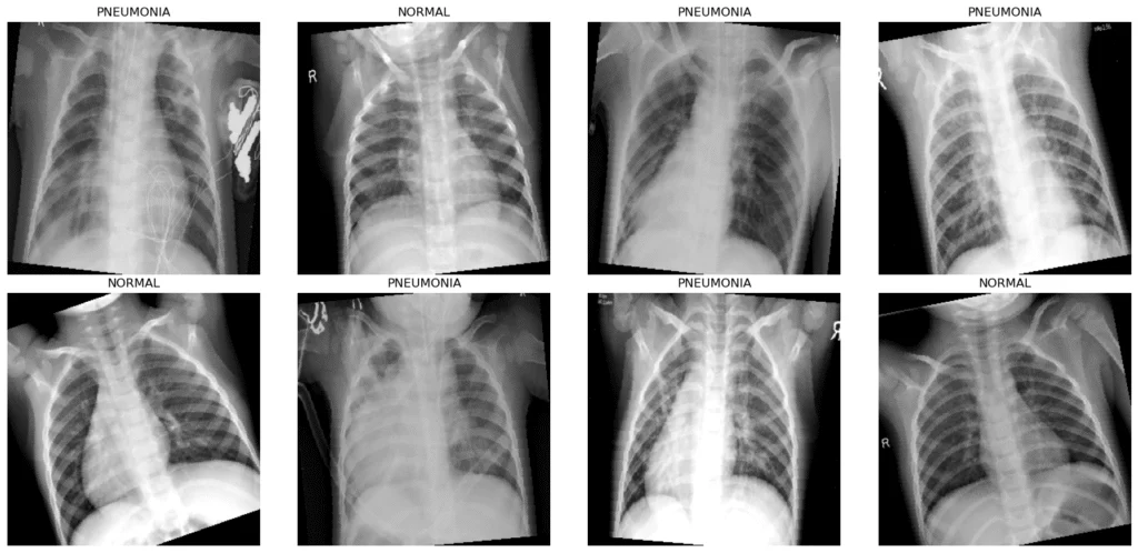
images, labels = next(iter(train_loader))Loaded datasets - Train: 4832, Val: 400, Test: 624# Display a grid of the first 8 images from the batch along with their labels
visualizer.display_image_grid(images[:8], labels[:8])One augmented batch of training films
Initialize network and trainer
# Initialize the PneumoniaClassifier model with the given configuration and move it to the specified device
model = PneumoniaClassifier(config).to(device)

# Log the model architecture
logger.info(model)

# Display a summary of the model architecture with input size details
summary(model, input_size=(3, config.image_size, config.image_size))

# Initialize the ModelTrainer with the model, configuration, and device
trainer = ModelTrainer(model, config, device)Train the network
history = trainer.train(train_loader, val_loader)Starting training for 20 epochs
Epoch [1/20] | Train Loss: 0.2342 | Train Acc: 0.9123 | Val Loss: 0.1554 | Val Acc: 0.9400 | LR: 0.000300
Epoch [2/20] | Train Loss: 0.1312 | Train Acc: 0.9491 | Val Loss: 0.2454 | Val Acc: 0.9250 | LR: 0.000300
Epoch [3/20] | Train Loss: 0.1233 | Train Acc: 0.9505 | Val Loss: 0.1564 | Val Acc: 0.9450 | LR: 0.000300
Epoch [4/20] | Train Loss: 0.1137 | Train Acc: 0.9551 | Val Loss: 0.1124 | Val Acc: 0.9525 | LR: 0.000300
Epoch [5/20] | Train Loss: 0.1098 | Train Acc: 0.9570 | Val Loss: 0.1102 | Val Acc: 0.9675 | LR: 0.000300
Epoch [6/20] | Train Loss: 0.0952 | Train Acc: 0.9646 | Val Loss: 0.0960 | Val Acc: 0.9625 | LR: 0.000300
Epoch [7/20] | Train Loss: 0.0908 | Train Acc: 0.9632 | Val Loss: 0.1239 | Val Acc: 0.9600 | LR: 0.000300
Epoch [8/20] | Train Loss: 0.0920 | Train Acc: 0.9656 | Val Loss: 0.1111 | Val Acc: 0.9625 | LR: 0.000300
Epoch [9/20] | Train Loss: 0.0902 | Train Acc: 0.9644 | Val Loss: 0.1156 | Val Acc: 0.9625 | LR: 0.000300
Epoch [10/20] | Train Loss: 0.0776 | Train Acc: 0.9673 | Val Loss: 0.1166 | Val Acc: 0.9525 | LR: 0.000150
Epoch [11/20] | Train Loss: 0.0749 | Train Acc: 0.9714 | Val Loss: 0.0892 | Val Acc: 0.9725 | LR: 0.000150
Epoch [12/20] | Train Loss: 0.0738 | Train Acc: 0.9737 | Val Loss: 0.0870 | Val Acc: 0.9625 | LR: 0.000150
Epoch [13/20] | Train Loss: 0.0675 | Train Acc: 0.9760 | Val Loss: 0.0922 | Val Acc: 0.9625 | LR: 0.000150
Epoch [14/20] | Train Loss: 0.0672 | Train Acc: 0.9766 | Val Loss: 0.1025 | Val Acc: 0.9575 | LR: 0.000150
Epoch [15/20] | Train Loss: 0.0663 | Train Acc: 0.9727 | Val Loss: 0.0976 | Val Acc: 0.9650 | LR: 0.000150
Epoch [16/20] | Train Loss: 0.0591 | Train Acc: 0.9762 | Val Loss: 0.1300 | Val Acc: 0.9600 | LR: 0.000075
Epoch [17/20] | Train Loss: 0.0612 | Train Acc: 0.9785 | Val Loss: 0.1122 | Val Acc: 0.9625 | LR: 0.000075
Epoch [18/20] | Train Loss: 0.0624 | Train Acc: 0.9752 | Val Loss: 0.0987 | Val Acc: 0.9700 | LR: 0.000075
Epoch [19/20] | Train Loss: 0.0612 | Train Acc: 0.9781 | Val Loss: 0.0946 | Val Acc: 0.9675 | LR: 0.000075
Epoch [20/20] | Train Loss: 0.0593 | Train Acc: 0.9774 | Val Loss: 0.0786 | Val Acc: 0.9700 | LR: 0.000075Plot model training and validation metrics across epochs
trainer.plot_training_history()Loss and accuracy across 20 epochs
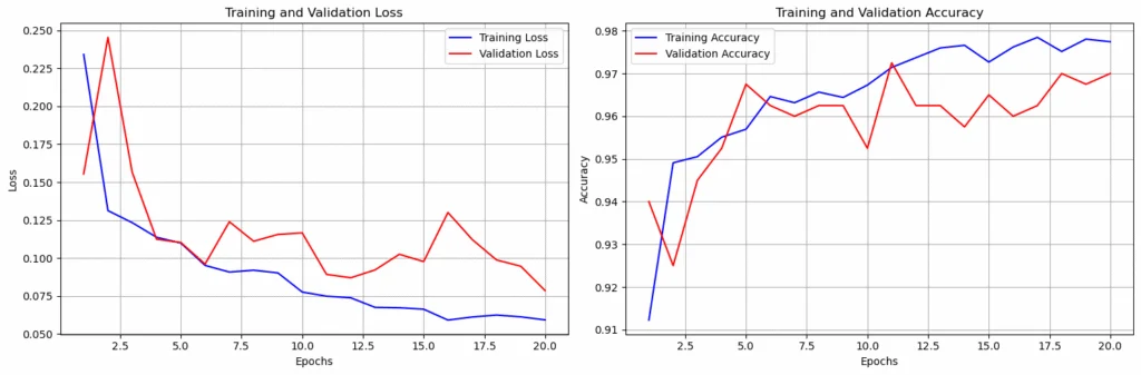
The training log does not end on a plateau. The lowest validation loss falls in the final epoch, which means the run ended on its epoch budget and more epochs might still have helped. It also means the final weights are the best-by-validation checkpoint, and since the evaluation cell reloads a saved checkpoint only when the trainer has not been fitted in the session, the test metrics below come from these final-epoch weights. Training accuracy rises from 0.912 in the first epoch to 0.977 in the twentieth, and validation accuracy ends at 0.970 with the lowest validation loss of the run, 0.079, recorded in the final epoch. The learning rate falls from 3e-4 to 1.5e-4 at epoch 10, then to 7.5e-5 at epoch 16, each drop following four epochs without an improvement in validation loss.
The two curves stay close to one another, which is consistent with the model not overfitting the training split. The comparison is not exact. Training accuracy is measured on augmented images while the weights are still changing, and validation accuracy on deterministic ones after the epoch ends. Whether it transfers to patients it has never seen is a different question, and the held-out test set is what answers it. The next stage runs it.
Assess model performance
if not hasattr(trainer, 'best_val_loss') or trainer.best_val_loss == float('inf'):
    trainer.load_checkpoint("best_pneumonia_model.pth")

test_loss, test_accuracy, metrics = trainer.evaluate(test_loader)
print(f"Test Accuracy: {test_accuracy:.4f}")
print(f"Test Precision: {metrics['precision']:.4f}")
print(f"Test Recall: {metrics['recall']:.4f}")
print(f"Test F1 Score: {metrics['f1_score']:.4f}")Test Accuracy: 0.8830
Test Precision: 0.8514
Test Recall: 0.9846
Test F1 Score: 0.9132Visualize model predictions
# Define the indices of the test dataset to visualize predictions for
indices = [4, 6, 285, 300]

# Iterate through the selected indices
for idx in indices:
    # Retrieve the image and its corresponding label from the test dataset
    image, label = test_dataset[idx]

    # Add a batch dimension to the image tensor and move it to the specified device (e.g., GPU or CPU)
    image_tensor = image.unsqueeze(0).to(device)

    # Disable gradient computation for inference
    with torch.no_grad():
        # Pass the image through the model to get the output logits
        output = model(image_tensor)

        # Apply softmax to convert logits into probabilities
        probabilities = F.softmax(output, dim=1)

    # Visualize the image along with the predicted probabilities and true label
visualizer.visualize_prediction(image, probabilities, label)Normal film predicted normal
A second normal film, less one-sided
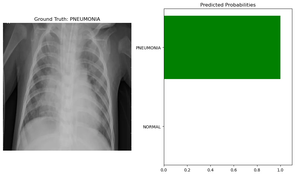
Pneumonia film predicted pneumonia
A second pneumonia film predicted pneumonia
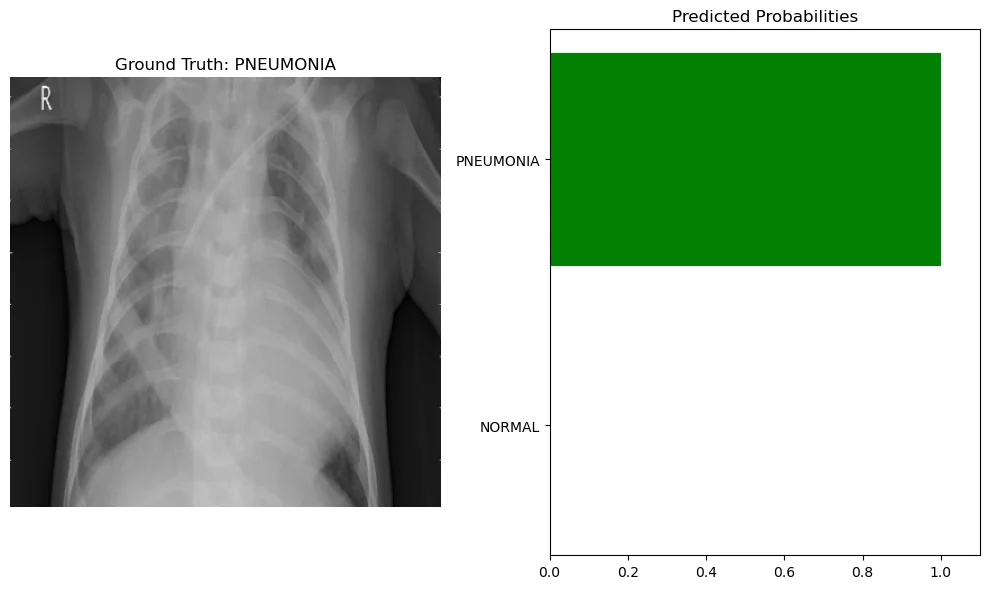
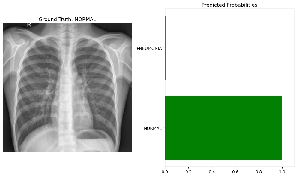
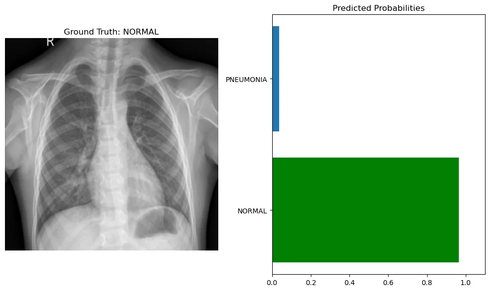
The four test images above are selected examples, and all four are classified correctly with almost all of the probability mass on the true class. Networks trained with cross-entropy commonly produce probabilities close to zero or one even when they are wrong, so predicted probabilities would need to be further analyzed for the other subjects in the test stratum.
Overall, this workflow illustrates a complete deep learning pipeline for medical image classification. The combination of configuration-driven design, modular components, checkpointing, and both quantitative and qualitative evaluation is a foundation for further experimentation. Further steps to refine this pipeline could include a calibration analysis, a decision threshold chosen for the intended screening role, evaluation across sites and equipment, and a review of the false positives that threshold produces.
Key Takeaways
Moving a model to the device shortens each trial by computing a step’s independent results in parallel. A sweep benefits because the same budget then covers more configurations, so the gain is in wider exploration, and nothing the model learns changes.
It depends on model size, batch size, tensor shapes, numeric precision, and whether the run is bound by arithmetic or by data loading. A figure measured on one pair of processors does not carry over to another, so treat any quoted speedup as specific to its setup.
Small models, small batches and low dimensional tabular data can finish sooner on a CPU, because the transfer and launch cost is never repaid. LoRA does not extend that to a large backbone. It cuts trainable parameters and optimizer state while the arithmetic stays close to where it was.
Validation reached 0.970 on 400 images from the same 5,232-image pool, and that split also chose the checkpoint and drove the schedule. The patient-independent test set gives 0.883, and that is the figure to read for unseen patients.
Recall of 0.985 against precision of 0.851 means the model caught nearly every pneumonia case and also flagged a substantial share of normal films. Which error costs more depends on the intended use, and four confident examples are not a calibration check.
The run fixes a seed of 42 for NumPy and PyTorch and sets the two cuDNN flags, which removes the largest sources of variation on one machine. Results can still move with a different GPU, a different CUDA or cuDNN version, or a nondeterministic operation.
Data & License
“Chest X-Ray Images (Pneumonia)” © 2018 Daniel Kermany, Kang Zhang & Michael Goldbaum, from “Labeled Optical Coherence Tomography (OCT) and Chest X-Ray Images for Classification,” Mendeley Data, v2 (doi:10.17632/rscbjbr9sj.2). The images were resized and normalized for training. Source: data.mendeley.com/datasets/rscbjbr9sj/2.License: Creative Commons Attribution 4.0 International (CC BY 4.0). Used with attribution; the images were modified (resized and normalized). CC BY 4.0
© 2025 Philip Sarajlic. All rights reserved for the article’s original text and figures; the third-party data remains under the license shown above.
Code examples in this article are licensed under the Common Public Attribution License Version 1.0 (CPAL-1.0), an OSI-approved copyleft license based on the Mozilla Public License 1.1. Initial Developer: Philip Sarajlic.
Attribution required by CPAL Exhibit B: © 2025 Philip Sarajlic · “Based on code by Philip Sarajlic” · philipsarajlic.com · no graphic image. This attribution must be displayed in Larger Works.
Modifications must be released in Source Code form under CPAL-1.0. Making the code usable by anyone other than you over a network is External Deployment under the license and is treated as distribution, so the Source Code must be made available to those users.
Full text: opensource.org/license/cpal-1-0 (SPDX identifier CPAL-1.0)